The Neural Network, Demystified

Neural networks have achieved amazing performance in many ML/AI related tasks, such as speech recognition, computer vision, and NLP. Their popularity as powerful classification and regressive tools mean that many beginners often encounter them when first getting introduced to ML.
Unfortunately, such individuals, myself included, often found themselves completely lost in the complexity of the Neural Network (NN) jargon itself — layers, neurons, activation functions, dropout, etc. Whenever we get an idea to pursue, we then have to rely on random tutorials which often are unrelated to the topic, randomly applying options and hoping the model functions as expected.

In this guide, I hope to introduce NNs in a far more intuitive form — math. By the end, you should have a much better conceptual understanding of NNs and how to approach implementing them in your projects.
Agenda
- Structure
- Training
Structure
The Perceptron
The first step to understanding NNs is to understand what they are made up of — neurons.
An artificial neuron in NNs functions similarly to biological neurons in our body by taking input, processing it, and producing some output.
An example of such a neuron is the Perceptron.

The perceptron follows the following formula to calculate outputs based on inputs.

Remember that x1 and x2 are inputs, w1 and w2 are the respective weights for the input, and b is a bias offset (constant).
The “y” value is then given as input into the Limiter, which is essentially a Heaviside/Step Function. In this way, the output of a Perceptron is always 0 or 1. Note that the threshold is the lowest necessary “y” value for the perceptron to output a 1 — for a regular Heaviside function, the threshold would be 0.
For example, lets say we want to mimic an AND logic gate using a perceptron.

A two input AND gate outputs a 1 only if both inputs are 1. Next, lets say that our perceptron looks like this:
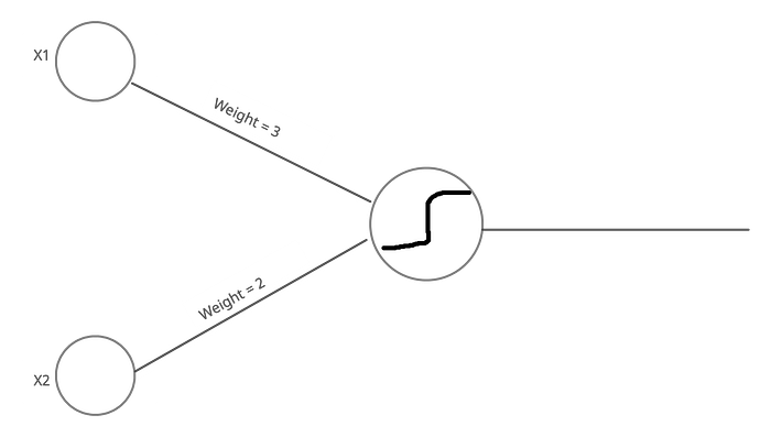
If both inputs are 1, the weighted sum is 5 (1 * 3 + 1 * 2). Therefore, the threshold of the limiter must be 5 as well, as the limiter should only output 1 if the input is at least 5.
One important characteristic of the Perceptron given above is that the weights of each input are not equal. This means that the value of input x1 has a greater impact on the output as compared to x2 — or the Perceptron is more sensitive to x1.
With an understanding of how a neuron functions, its evident that for the vast majority of tasks, a single neuron is not sufficient. For this reason, multiple neurons are connected into a Neural Network.

To clarify common NN vocabulary using the above image:
Layer — Each individual column of neurons. Not connected to each other but each one is receiving the same input as the other neurons in the same layer and sends output to each neuron in the next layer.
Input Layer / Output Layer — Blue column of neurons and green column of neurons respectively. Data starts at the input layer and the network’s classification/regression is given at the output layer.
Hidden Layers — Black columns of neurons in the middle. Essentially layers between input and output.
Dense Layer — A layer where each neuron is connected to every single neuron from the previous layer. Each layer in the image is a Dense Layer.
Input Dimension — Number of input features/data points (ex. 4 for the first hidden layer) for a layer.
Units — Number of neurons in a layer.
Activation Function — Defines what function a neuron should use to process and convert input to output (ex. a Perceptron uses Heaviside/Step Function, but other neurons can use ReLU, sigmoid, etc.). This is user configurable.
Weights /Parameters— The strength of the connection between two neurons, visualized as the line connecting them.
Lets wrap up this section with simple example. Let’s say I wanted to create a neural network that functioned like a XOR gate.
from keras.models import Sequentialfrom keras.layers import Denseimport numpy as npmodel = Sequential()
model.add(Dense(units=16, activation='relu', input_dim=2))
model.add(Dense(units=1, activation='sigmoid'))training_data = np.array([[0, 0], [0, 1], [1, 0], [1, 1]], "float32")
training_target_data = np.array([[0], [1], [1], [0]], "float32")
test_data = np.array([[1, 0]], "float32")
test_target_data = np.array([[1]], "float32")
The model has input layer and output layer, defined in lines 8 and 9. The first layer has 16 neurons, an input dimension of 2 (since each training data sample has 2 data points), and a ReLU activation function. The second layer (output) has one neuron and sigmoid activation function to provide the output. The model structure is visualized below.

One important point to remember is that NNs refer to a group of similar models that can vary in structure slightly and focus on different ML related tasks (CNN, RNN, LSTM, etc.). The type of NN explained in this section is the simplest, called the ANN. However, ANNs are the most fundamental of the NNs and enough for many tasks. They also allow for easier understanding of each variation.
Training
With the foundational concepts of NNs covered, this section will explain the crux of how/why the model is so effective in learning from data.
A short note — Deep Learning relies heavily on calculus concepts so a strong understanding of the fundamentals (derivatives, gradients, etc.) makes the ideas easier to grasp.
The Cost Function
The basis of training is the Cost Function, which is a measure of error between what the model predicts and the actual output value. It is calculated using the following formula, where n is the total number of training samples, i is an individual training sample, and f represents the NN.

Note that the terms “Cost Function” and “loss” are used almost interchangeably — “loss” just refers to the error value on one training sample rather than the whole dataset.
In the previous section, weights/parameters were introduced as a measure of the connection strength between 2 neurons, visualized as a line connecting them. Prior to training, weights are given random values.
The goal of training a model is to modify the weights/biases until the Cost Function is minimized.
In simpler terms, keep adjusting the weights until the model’s predictions are as close as possible to the real values in the dataset.
Forward/Back Propagation
Assume the model above is attempting to classify an input image as a number from 1–4. Note there are 4 output neurons signifying the confidence (0–1) that an input image is each number in the range.
When a training sample enters the network, data moves from left to right across the model’s layers — this is called forward propagation. At the end, the data is classified and the loss is calculated.
Using the loss for that specific training example, weights/biases for all layers are modified through a technique called back propagation. This does not only involve increasing or decreasing them — it also involves calculating what relative proportions to those changes cause the most rapid decrease to the Cost Function of the network.
For example, let’s say that an input image of a 2 is given to the model and the following output is produced:

The model’s confidence in the correct class (2) is lower than another class (3).
An intuitive way to increase the “2” neuron’s activation output may be by increasing the output of the activations functions of the neurons in the previous layer, since this is what the model’s output neuron receives as input.
However it is impossible to directly change the activation output, as it is a predefined function.
Instead, the weights and biases connecting the last hidden layer to the output layer must be modified in a manner that increases the activation output of the “2” neuron and ultimately decreases the Cost Function. To do this, the weights and biases connecting to the layer prior to the last hidden layer must be modified as well. In this way, the changes are propagated backwards.
This paragraph will provide a more in-depth, mathematical look into back propagation. It is not necessary to understand this in order to comprehend how training works and so can be skipped if the calculus concepts are unfamiliar.
Let’s take a neural network with 4 layers and 1 node in each layer.

The last 2 nodes are called a^(n-1) and a^(n). (note that the superscripts denote the neuron numbers and not exponents). Let w^(n) be the weight connecting a^(n-1) and a^(n) and b^(n) be the bias. Remember that:

In order to decrease and eventually find the minimum of the Cost Function, it is imperative to first find how sensitive the Cost Function is to small changes of the weights in the network. This is done starting at the nearest weight to the output, or w^n in this case.
Since sensitivity is essentially describing the derivative, the goal is to find the ratio of the derivative of the Cost Function to the derivative of the weight function. Using chain rule, this can simplified:

This is then repeated to test biases instead of weights. Then, the whole process is replicated for every single weight and bias in the network so weights/biases can be modified in while taking into account the impact of such changes on the Cost Function. It is with this technique that NNs maintain a high degree of accuracy in many tasks.
When to finish training?
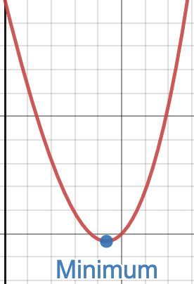
Generally, the model should finish training when the Cost Function is at a minimum (convergence). An example is shown below:
This can be done by setting arbitrary hyperparameters, graphing model performance once training is finished and tweaking hyper parameters repeatedly until the model performance is best.
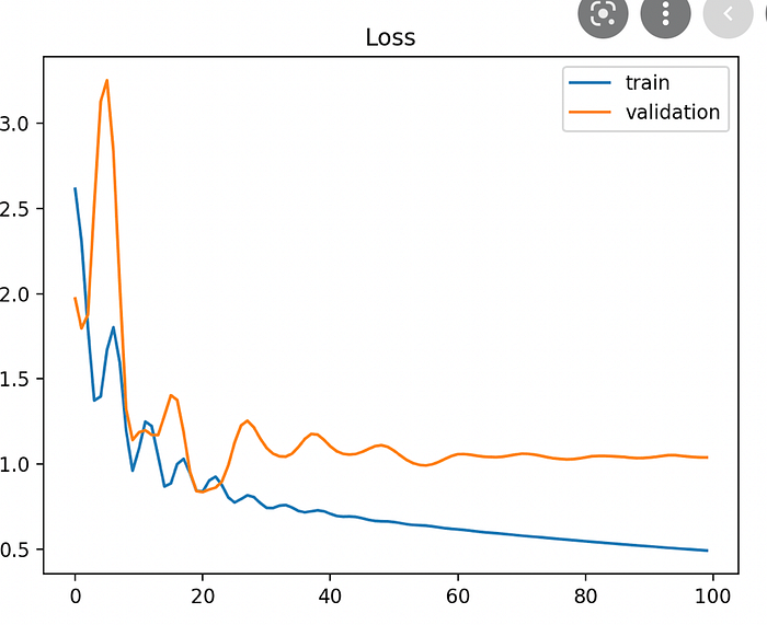
However, this strategy can lead to overfitting where the model performance on the training set is stellar but the parameters conform to closely to the data, causing higher loss in test datasets.
To prevent this, it is vital to segregate a small portion of the training set as the validation set and check the Cost Function on this set for each iteration of training to prevent overfitting. Then, take the hyper parameters that minimize loss on both training and validation datasets for the final model.
Hyperparameters
Hyperparameters are user-configurable options that control the training process. Tuning them is a vital part of achieving a model which performs well and can often only be done empirically. Below is a list of common hyperparameters and their effects on how the model learns.
- Train-test split ratio: Perhaps the most common hyper parameter, the train-test split ratio decides how much of the dataset should be allocated for training and testing. Common values include 60%–40% or 70%–30% but other ratios are used as well. The main factor to keep in mind is that a balance between training and testing sets should exist such that the model trains without overfitting and there is sufficient test data to gain an accurate picture of model’s performance.
- Learning rate: One of the most important hyperparameters, learning rate corresponds to how much the model’s weights should be changed every time the model’s cost function is calculated after each training sample. A high learning rate means that weights are modified aggressively to find the minimum of the Cost Function as soon as possible, but this can lead to unpredictably when the parameters sway wildly every epoch or the minimum of the Cost Function is passed. Conversely, a lower learning rate means that weights are modified in a more minute manner, but this can lead to the model taking longer to train and performance increase becoming stagnant.
Therefore, it takes experimentation to find the best learning rate. However, they are generally a very small positive value in the range 0–1.
Additional information can be found here:
https://machinelearningmastery.com/understand-the-dynamics-of-learning-rate-on-deep-learning-neural-networks/ - Optimization Algorithms: Optimizers are methods in which the model changes the weights/biases in response to the cost function. There are many different techniques that be used but many require a more in depth explanation to fully understand how they impact a NN.
This article explains the various types of optimizers more in depth: https://towardsdatascience.com/optimizers-for-training-neural-network-59450d71caf6 - Choice of activation function: Recall that each layer has an activation function which serves to compress/process the weighted input into a desired output range. Examples of such functions include ReLU, Softmax, and Sigmoid.
Generally, hidden layers all use the same activation function to ensure consistency across middle network processing. The activation function used for NNs is most commonly ReLU for a variety of reasons, most importantly its ability to combat the vanishing gradient issue. A graph of the ReLU function is below (formula is max(0.0, x) )
Output layers have activation functions that match the type of ML problem the model aims to solve. For example, classification problems often use a sigmoid function while regressive problems will require a linear output function.


- Number of hidden layers/units: The main guidelines to follow regarding this topic is that for the vast majority of tasks, there should be no need for more than 2 hidden layers. Additionally, each hidden layer should have a size between the sizes of input and output layers (so mean of input/output units is commonly used). The performance increase from adding more layers/units than this is minimal/nonexistent.
Final Thoughts
Hopefully, this article served to induce a strong conceptual understanding of the “how” and “why” of NNs. There are numerous variations to explore such as RNN and LSTM that specialize in solving different types of ML/AI problems.
Thank you for reading! If it helped, please consider connecting on LinkedIn — I’d love to hear your thoughts.